Binomial risk under absolute value loss: why a cauliflower?

If \(X \sim \text{Binom}(n,p)\) then the estimator \(\hat{p} = X/n\) satisfies \(\mathbb{E}(\hat{p} - p)^2 = n^{-1}p(1-p)\), which is quadratic (and concave) in \(p\). Instead of using a squared error, we could consider the risk under the absolute value loss:

\[ R(p) = \mathbb{E} | \hat{p} - p| \]

Below, we plot the risk \(R\) for \(n = 4,5,10\) and observe an interesting pattern: the risk is not concave and has a cusp at \(k/n\). This is much different than the squared error loss!

R <- function(n,p) {
  x <- 0:n
  px <- dbinom(x, size=n, prob=p)
  sum(abs(x/n - p)*px)
}

library(ggplot2)

Warning: package 'ggplot2' was built under R version 4.3.1

n <- c(4,5,10)
p <- seq(0,1,by=0.01)

df <- expand.grid(n=n, p=p)

df$Rp <- apply(df, 1, function(row) R(row[1], row[2]))

df$n <- as.character(df$n)

p <- ggplot(data=df,aes(x=p, y=Rp, color=n)) + geom_line() + 
  theme_bw() + 
  xlab("p") + 
  ylab("Risk")

print(p)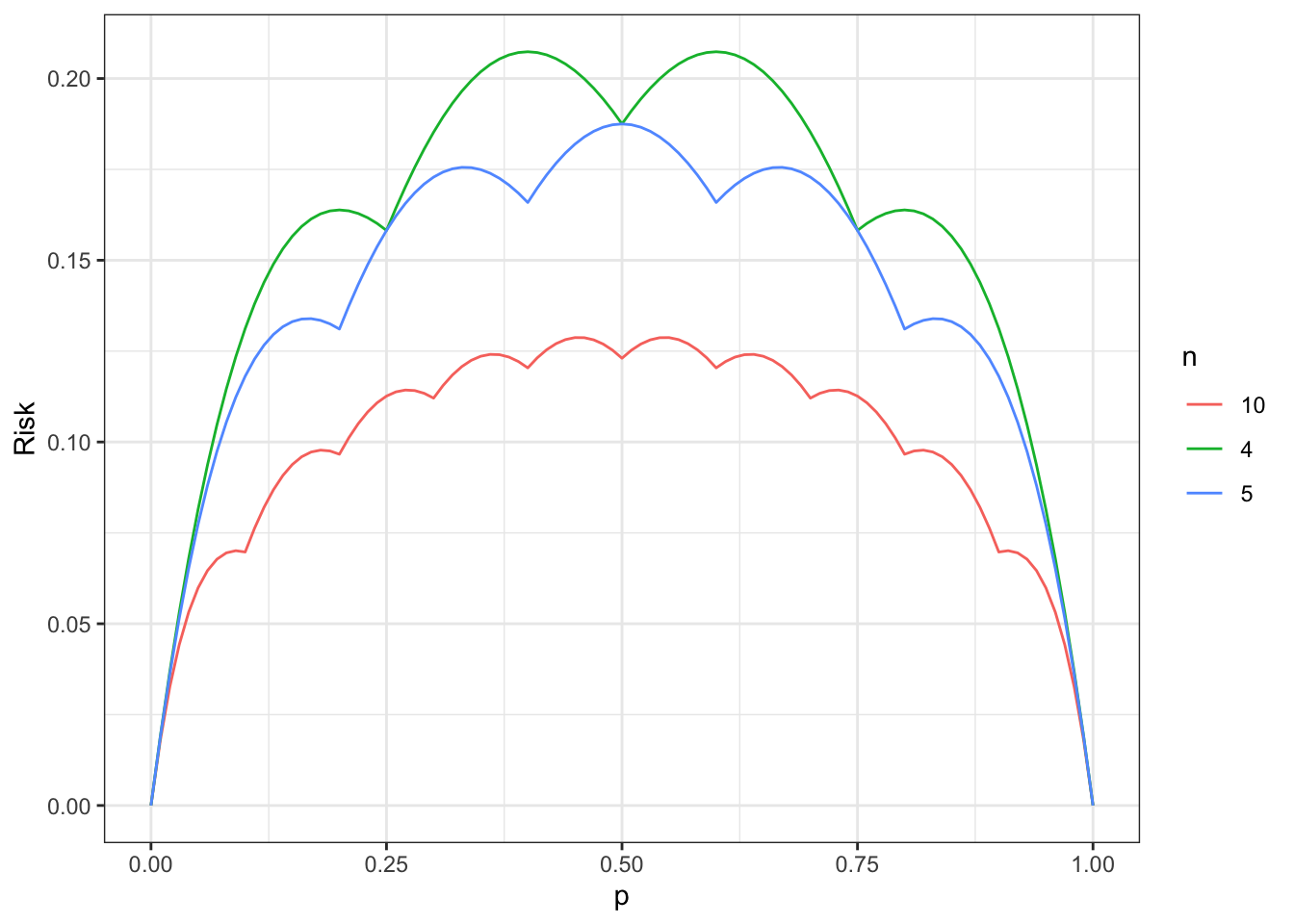

The above is the same as the one which was apparently hand-drawn in Blyth (1980).

We can also prove the following result: for \(\frac{k-1}{n} \leq p \leq \frac{k}{n}\):

\[ R(p) = 2 \binom{n-1}{k-1} p^k (1-p)^{n-k+1} \]

This is exercise 1.13 in Lehmann and Casella (1998). We can demonstrate this quickly for \(k = 1\):

\[ \begin{align} R(p) &= p(1-p)^n + \sum_{x=1}^n \left(\frac{k}{n} - p \right) p^x (1-p)^{n-x} \\ &= p(1-p)^n + \mathbb{E}(\hat{p} - p) + (1-p)^n p \\ &= 2(1-p)^n. \end{align} \]

Moreover, by differentiating \(R(p)\) in this range, we see

\[ R'(p) = 2(1-p)^n - 2np(1-p)^n. \]

Setting this equal to \(0\) and solving for \(p\) yields \(1/(n+1)\). I.e., the critical point in \([0, 1/n]\) on the above plot occurs at \(1/(n+1)\) .

References

Blyth, C. R. (1980). Expected absolute error of the usual estimator of the binomial parameter. The American Statistician, 34(3), 155-157.

Lehmann, E. L., & Casella, G. (1998). Theory of point estimation. New York, NY: Springer New York.