Slide-seq Mouse Hippocampus • MorphoGAM

In this analysis, we will use MorphoGAM to analyze CA3 cells in the mouse hippocampus.

First, we load the necessary packages.

library(MorphoGAM)
library(dplyr)
library(STexampleData)
library(igraph)
library(tidyverse)

Next, we load the data and remove outlier points:

spe <- STexampleData::SlideSeqV2_mouseHPC()
#> see ?STexampleData and browseVignettes('STexampleData') for documentation
#> loading from cache

ixs <- which(spe$celltype == "CA3") #subset to CA3

xy <- spatialCoords(spe)[ixs,]
Y <- counts(spe)[,ixs]

xy.dist <- as.matrix(dist(xy))
knn <- 20
prune.outlier <- 3
nnk <- apply(xy.dist, 1, function(x) sort(x)[knn+1])
outlier <- which(nnk > (prune.outlier)*median(nnk))

xy <- xy[-outlier,]; Y <- Y[,-outlier]

data.frame(x=xy[,1], y=xy[,2]) |> ggplot(aes(x=x,y=y)) + 
  geom_point(size=0.5) + theme_bw()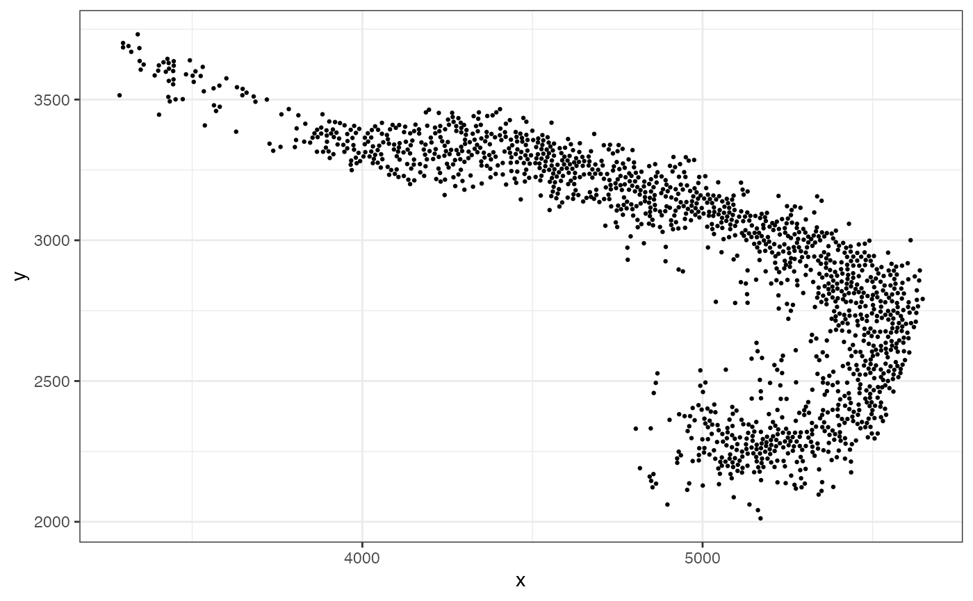

Now, we can fit a 1D curve passing through and observe the resulting coordinates:

fit <- CurveFinder(xy)
fit$curve.plot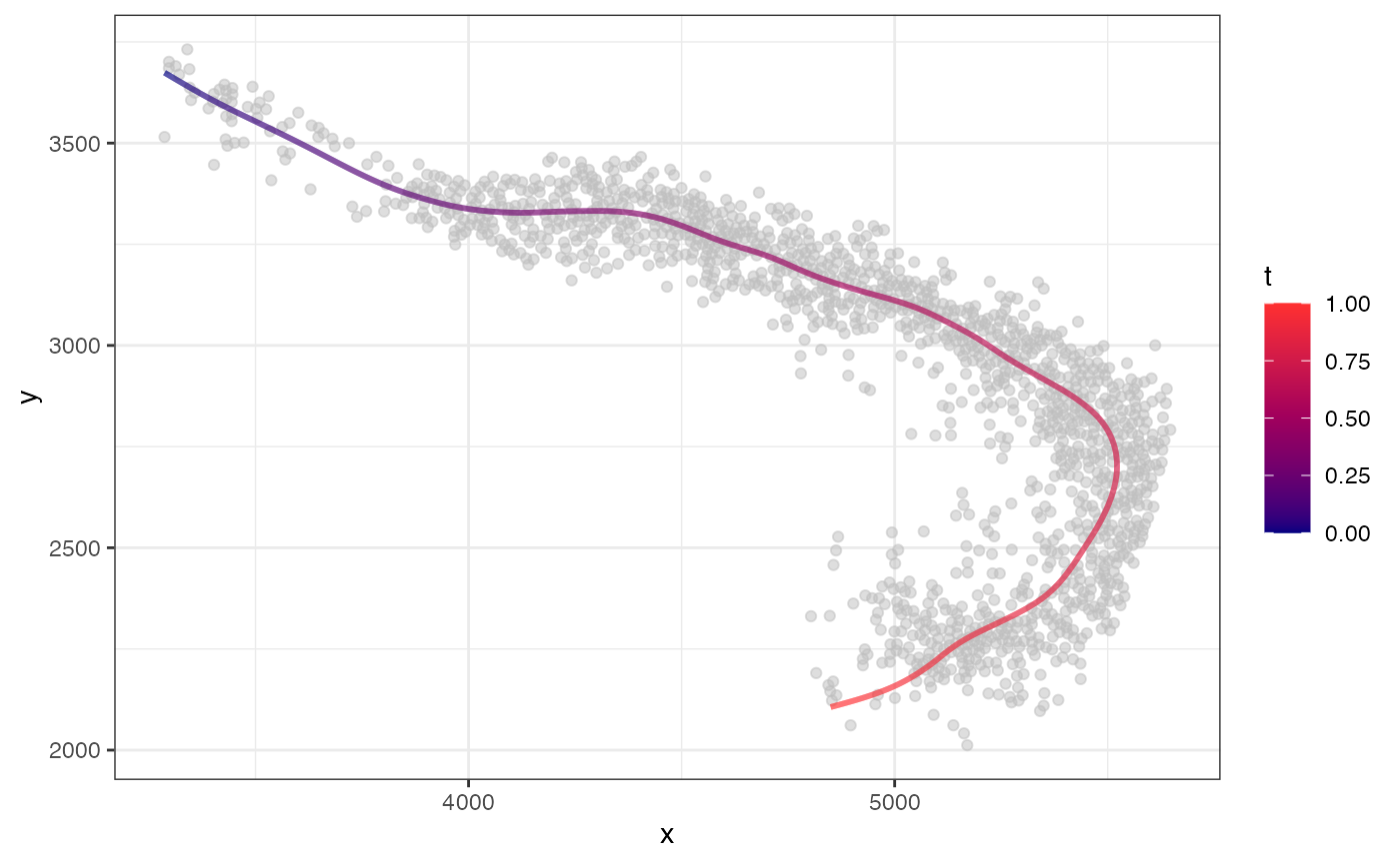

fit$coordinate.plot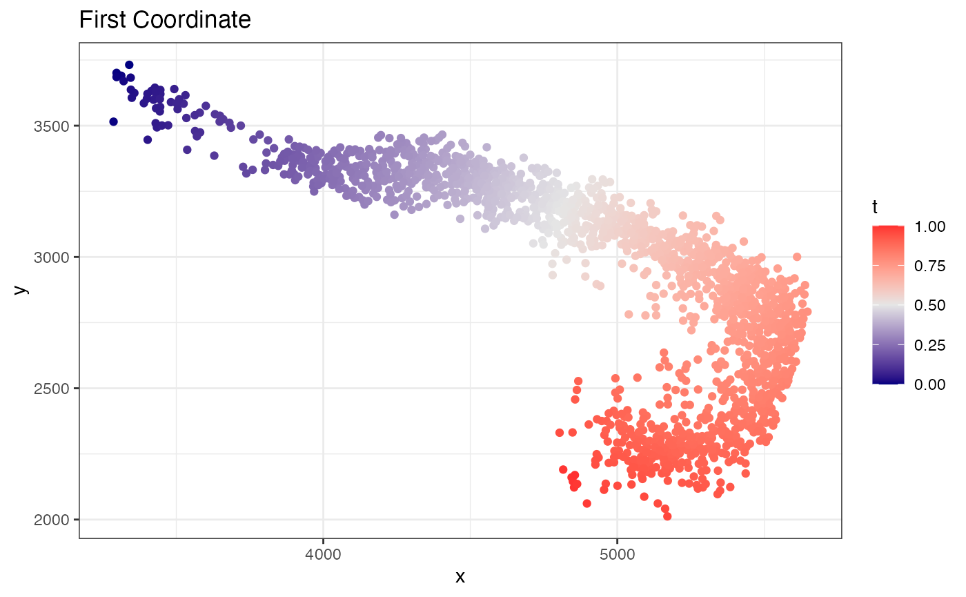

fit$xyt also includes the values. Now to find variable genes along this path, we can use the MorphoGAM() function. For speed, let’s first subset to 2000 variable genes

# Find 2000 variable genes based 

logCPM <- log2(1e6*(Y/Matrix::colSums(Y)) + 1)
var.genes <- names(sort(apply(logCPM, 1, var), decreasing=TRUE))[1:2000]

Y <- as.matrix(Y[var.genes,])

Now we fit the model. In the design argument, we specify that we want a model that fits a smooth function to both the $t$ (first coordinate) and $r$ (second coordinate).

mgam <- MorphoGAM(Y, curve.fit=fit,
                  design = y ~ s(t) + s(r))
#> ================================================================================

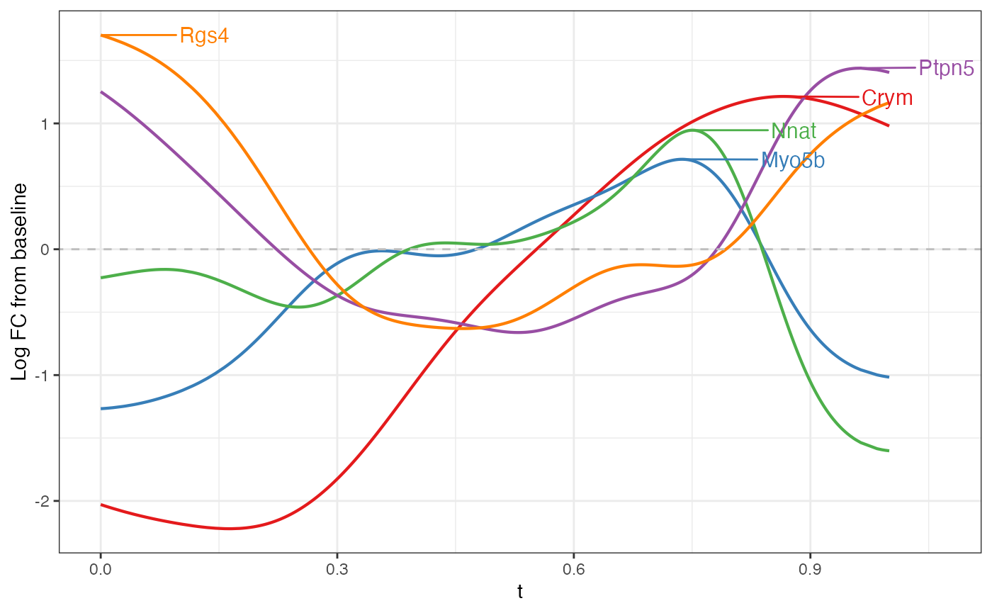
The first thing we can do is look at genes with a large peak in the $t$ direction. Here, the peak statistic is defined as the maximum log fold change from the baseline.

mgam$results |> arrange(desc(peak.t)) |> head()
#>          peak.t   range.t pv.t     peak.r     range.r          pv.r intercept
#> Rgs14  2.688307 0.5387266    0 0.06277392 0.002950812  4.016183e-02 -9.614966
#> Crym   1.827735 0.8088010    0 0.32335465 0.104397880  5.124054e-04 -7.573050
#> Fxyd7  1.659239 0.1689494    0 0.00000000 0.000000000  8.469104e-01 -8.702739
#> Necab2 1.413801 0.3406113    0 0.05697628 0.010565701  4.310323e-02 -8.679102
#> Nptx1  1.391123 0.4382267    0 0.12000145 0.053388796  3.192286e-02 -7.406455
#> Bok    1.355025 0.3707605    0 0.23728096 0.157378967 -1.169573e-06 -7.389233

top6 <- mgam$results |> arrange(desc(peak.t)) |> head() |> rownames()

Note that any list of genes can always be plotted with plotGAMestimates().

plotGAMestimates(Y, genes=top6, curve_fit=fit, mgam_object=mgam, nrow=2)

Repeating the same for the $r$ direction:

top6 <- mgam$results |> arrange(desc(peak.r)) |> head() |> rownames()

plotGAMestimates(Y, genes=top6, curve_fit=fit, mgam_object=mgam, nrow=2, type="r")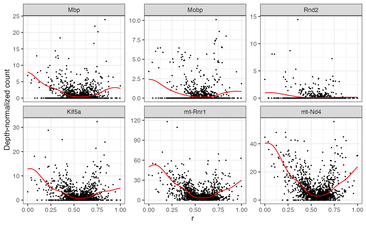

Note that these statistics are defined for convenience, but the entire function is available in the output of MorphoGAM(). Example, with Rgs14 gene:

gene <- "Rgs14"

fitted_function <- mgam$fxs.t[gene,]

data.frame(x=fit$xyt$t, y=fitted_function) |> ggplot(aes(x=x,y=y)) + 
  geom_line(color="blue") + theme_bw() + geom_hline(yintercept = 0, linetype="dashed") + xlab("t") + ylab("LogFC from baseline")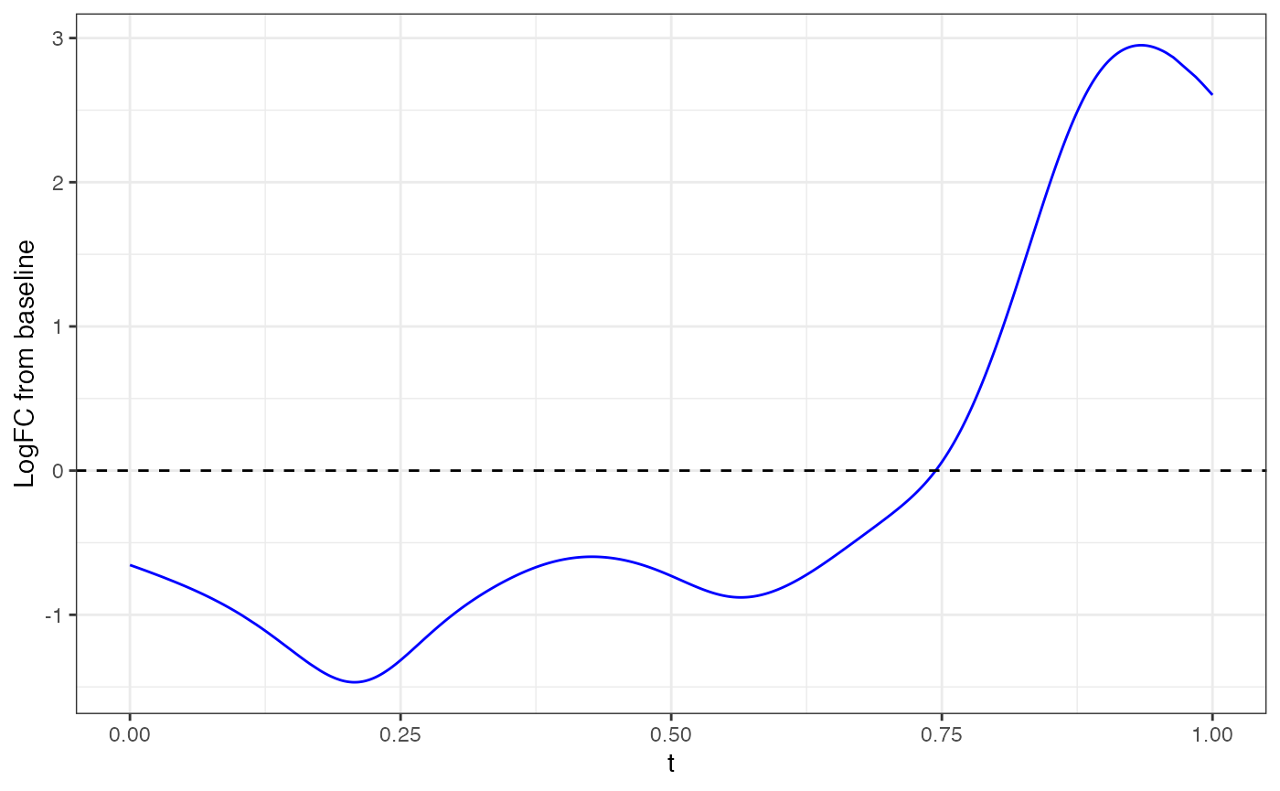

Finally, we can look at the FPC loadings. Here, we plot the second FPC loading in the $t$ direction.

plotFPCloading(mgam_object = mgam,
               curve.fit = fit,
               L=2)